Kevin Chao
Data Scientist

CrazyTremor: A MATLAB GUI for examining triggered tremor
Updated: April, 10, 2024
- Published source codes on Mathworks File Exchange (download link).
- Updated emails and SAC files download link
(1) About CrazyTremor:
1.1 Introduction:
CrazyTremor is a MATLAB package for searching for triggered tremor or triggered earthquakes
from a sizeable seismic dataset. It was developed by Dr. Chunquan Yu and Dr. Kevin Chao.
1.2 Publication:
Chao, K. and C. Yu (2018), A MATLAB GUI for Examining Triggered Tremor: A Case Study in New Zealand, Seismol.
Res. Lets., doi:10.1785/0220180057. [PDF]
Snapshot of CrazyTremor - 1

Snapshot of CrazyTremor - 2
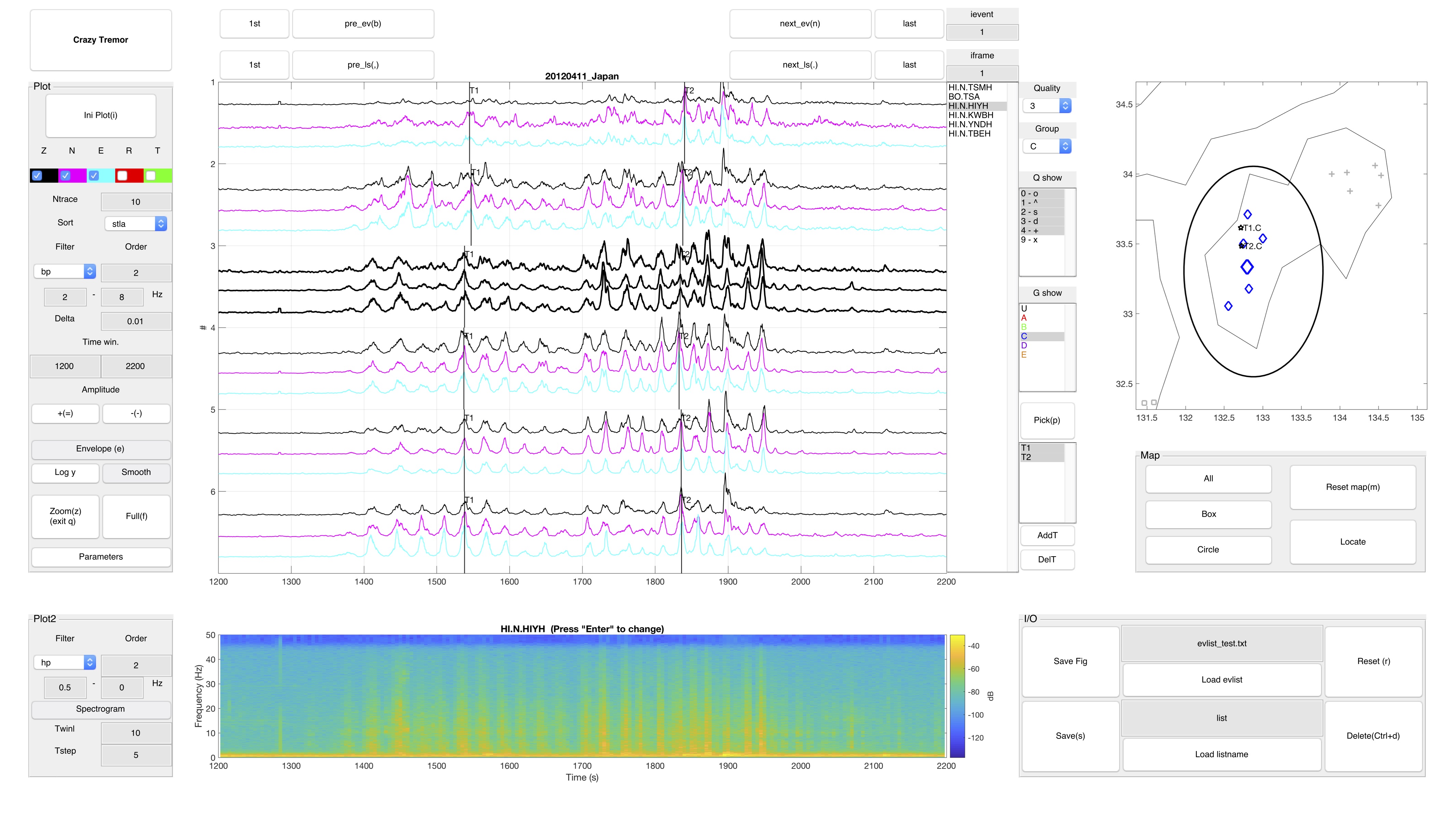
1.3 Important features:
-
Multiple channels:
The main function screen shows the tremor-band seismograms of triggered tremor, surface-wave-band
seismograms or spectrograms for comparison, and a station map.
-
Tag function:
Users can select different triggering events and classify each station with quality and/or group.
The tagging results will show on the station map for clearer visualization of the examined outcome.
-
Location of tremor sources:
Users can manually pick the arrival times of individual tremor bursts and quickly obtain preliminary locations.
(2) Download CrazyTremor (version 1.1.2024):
(3) Data preparation:
3.1 System requirements:
-
MATLAB in Mac, Windows, or Linux; versions 2018a, 2017b, 2017a, 2016b, or 2016a (MATLAB download page)
-
Toolbox requirements: Signal Processing and Mapping
3.2 Prepare seismic data in a SAC (seismic analysis code) format:
-
Assign each seismic waveform in a SAC format a consistent file name:
"NETWORK.NAME.TYPE.SAC” (e.g., NZ.BKZ.HHZ.SAC)
-
Place SAC files in a sub-directory folder under a main "SAC" folder in the working directory.
Example:
> Download test SAC files link-1 (i.e., waveforms for triggered tremor in Japan, Chao and Obara, JGR, 2016)
> Place the downloaded SAC folder (i.e., SAC/demo_20120411_Japan) under directory ~/CrazyTremor_2018_v1.1/
~/CrazyTremor_2018_v1.1/SAC/demo_20120411_Japan
-
The default acceptance instrumental code includes BH, HH, EH, and SH in E, N, and Z (or U) components,
but the script will not read non-oriented components (i.e., 1 and 2).
-
Tip: We suggest preparing SAC files for only a few hours, for instance, two hours of data or less if the earthquake
epicentral distance is within 10,000 km of the study region.
3.3 Create header lists for all waveforms in MATLAB:
-
Once all sub-directories are placed under a main “SAC” folder in the working directory,
execute the “ct_gen_listname” script to generate header lists for all waveforms.
>> ct_gen_listname
(4) Open the GUI (Graphical User Interface) window:
4.1 Open the GUI window in MATLAB by executing the script below:
>> y_CrazyTremor_v1
4.2 Overview the control panels of GUI:

(i) Map: Shows all stations and tagged information.
(ii) Tremor-band seismograms: Show multiple waveforms in the frequency range of a 2-8 Hz band-pass
filter, a 5 Hz high-pass filter, or any customized frequency range.
(iii) Surface-wave-band seismograms: Show Love and Rayleigh waves or a spectrogram for a comparison
with tremor-band seismograms.
(iv) Switch: Switches between earthquake events and lists of seismograms.
(v) Input and output: Saves the examination results and outputs snapshots to a PDF file.
(5) Load the data
5.1 Click “Reset map (m)” to load waveform information.
-
All stations in the first folder (first event) will appear on the map.
-
If a saved header exist (i.e., the file 'list_o', see 11.6), it will load
the latest saved information.
(6) Select stations
6.1 Click "All" to select all stations.
6.2 Click "Box" and click two points (diagonal points) on the map
to select stations.
6.3 Click "Circle" and click two points (center and circle boulder)
on the map to select stations.
6.4 Default parameters: stations on the map that can be selected:
Quality (Q): all included (0, ,1, 2, 3, 4, 9)
Group (G): all included (U, A, B, C, D, E)
6.5 Zoom in zoom out of the map:
Use the MATLAB default “zoom in (⊕)" and “zoom out (⊖)"
function to adjust the size of the map (see the figure below).

(7) Plot waveforms

7.1 Click "Ini Box(i)" to plot the seismograms.
7.2 Select station components to display in Window (ii) and Window (iii). Default parameters:
Z, N, E components.
-
Click to modify the shown components.
7.3 Select the number of stations to display in Window (ii). Default parameters:
10 stations.
-
Change the number of stations to plot.
-
Tip: Show no more than 60 traces for faster examination.
(e.g., 20 stations with three components or 60 stations for one component.)
7.4 Select the frequency band for tremor-band seismograms. Default parameters:
2 - 8 Hz bp (band-pass) filter
-
Change waveforms to 5 Hz hp (high-pass) filtered seismograms:
In "Plot": Scroll down to the "bp" icon and change it to "hp"; then change the values
from "2" - "8" Hz to "5" - "0" Hz (i.e., apply the 5 Hz hp filter).
-
Tip: Use a 2-8 Hz band-pass filter for most cases and a 5 Hz high-pass filter only for
a mainshock epicentral distance of less than 3,000 km.
-
Select sampling rate (Delta) of the display seismograms. Default parameters:
0.1 second (or a 10 Hz sampling rate waveform)
-
Tip: For a more efficient analysis, CrazyTremor uses a default sampling rate of 0.1 seconds for displaying
seismograms in order to save the memory used in MATLAB. Change the display sampling rate with
a higher value on Window (ii) (for a higher resolution of tremor-band seismograms) and Window (iii)
(for a higher frequency range if the "spectrogram" function is selected, also see 7.9), depending on
the original data sampling rate, such as the following:
0.05 second (or 20 Hz )
0.02 second (or 50 Hz )
0.01 second (or 100 Hz )
7.5 Select raw seismograms (e.g., surface waves with a broadband station). Default parameters:
Not filtered.
-
Apply the lp (low-pass) filter on the reference-seismograms in order to show the
long-period waveforms (e.g., for a short-period station):
In "Plot": Scroll down to the "bp" icon and change it to "lp"; then change the values
from "0" - "0" Hz to "0.1" - "0" Hz (i.e., apply the 10 sec low-pass filter).
7.6 Zoom in and zoom out seismograms:
-
Click the seismograms:
7.6.1 Press the “Zoom (z)” icon (or “z” as a shortcut) and then click two points on any
seismogram (in either on window (ii) or window (iii)) with a mouse from left
to right to zoom in, “o” to zoom out, or “q” to quit the zoom-in and -out mode.
Tip: Press “q” to quit the zoom-in and zoom-out mode before proceeding to the next step.
7.6.2 Press the "Full(f)" icon (or "f" as a shortcut) to show the full length of the waveforms.
-
Enter values:
7.6.3 Input two values to show the fixed time window waveforms.
(e.g., 14,000 and 16,000)

7.7 Adjust the amplitude of the seismograms:
-
This option will change the waveform amplitude shown on
Window (ii) (apply to either filtered or envelope function seismograms) and
Window (iii) (apply to a regular seismogram, but not a spectrogram plot).

7.8 Display Envelope function of tremor-band seismograms (for Window (ii) only):
7.8a Change to display the envelope function: Envelope (e)
7.8b Change to smooth the envelope function: Smooth
Default smoothing parameter: 10
-
Change the "Smooth Timelength" to another value for smoother envelope function seismograms:
the larger the value, the smoother the seismograms. After changing the "Parameters"
(i.e., the value for a smooth time length), re-click the "Smooth" icon to re-plot the envelope function.
The envelop function shown above is smoothed with a time length of 5.
7.8c Change to display the logarithmic scale on the y-axis: Log (y):
7.9 Change to spectrogram plot (for Window (iii) only):
-
A user can choose to display the spectrogram instead of the surface waves with a selected station.
-
Tip 1: Apply a 0.5 Hz high-pass filter to avoid artificial noise generated by
long-period surface waves [Peng et al., SRL, 2011].
To apply:
In "Plot2": Scroll down the "bp" icon and change it to "hp" and change the values
to "0.5" - "0" Hz (i.e., apply a 0.5 Hz high-pass filter).
-
Tip 2: To display a higher frequency range (i.e., Nyquist frequency) on the y-axis of the spectrogram,
change the display sampling rate "Delta" from 0.1 seconds (10 Hz) (the Nyquist frequency is
5 Hz as a default) to a higher value (see section 7.4 for details).
(8) Tag stations with quality and group for each station
-
After determining the station quality, classify and
tag each station by a “Quality” (e.g., 0: not yet decided;
1: good; 2: maybe; 9: bad) and/or a “Group”
(e.g., A: source #1; B: source #2).
-
Note that the selected stations and tagging results will instantly appear on the map for more accurate visualization of station locations.
-
Tip: To examine a large number of seismic stations, start with a smaller area (e.g., 0.5 to 1 degree wide) and initially reject bad traces if no triggered signal traces appear (e.g., quality=9).

(9) Locate triggered sources
-
With this function, obtain quick preliminary locations for selected triggered bursts. The purpose of this locating
approach is to grid search the minimum root-mean-square value from differences between the theoretical and
observed travel times of S-waves as a triggered tremor source (see the Appendix in Chao et al., BSSA, 2013 for details).

9.1 Add "ticks":
-
Click "AddT" to add "tick" to each triggered event.
9.2 Pick an S-wave arrival time:
-
Select the number of ticks (e.g., click T1) and then click "Pick(p)." Then manually use the mouse to point
to the arrival times of an individual tremor source for each station. After the picking procedure, remember
to click the "q" key on the keyboard to quit the "picking mode."
-
After the initial picking, click the name of each station and use the left and right arrow keys on the
keyboard to adjust the arrival time.
-
Tip 1: To more easily pick the maximum point on the envelope function as an S-wave arrival,
apply "Envelope (e)" and then "Smooth" function on the tremor-band seismograms .
-
Tip 2: The locating script uses a general 1-D S-wave velocity model (see Figure to the right).
Change the velocity model to any localized values in the file at
~/CrazyTremor_2018_v1.1/utilities/vmodels/vmodel1.txt.
-
Tip 3: The locating script uses a fixed depth of 35 km to locate tremor.
Change default depth, find 'para.xdep = 35' in 'y_CrazyTremor_v1.m' for changing.
9.3 Get locations:
-
Click the "Locate" icon to instantly compute the best locations for selected "Ticks" and display the results
on the map. The script will also save a text file (file name: loc.txt) with the longitude and latitude information
under the event folder.
-
Tip: Use the error bars of the output location shown on the map and apply a move-out plot (see 10 below)
to judge whether the location is reliable or not.

(10) Generate a move-out plot
-
To generate a move-out plot (the farther the station from the source, the later the arrival) for all display seismograms:
In "Sort," scroll down the "stla" icon, and change it to "point"; then click a point on the map as the best location.
-
The tremor-band seismograms in Window (ii) will then be aligned based on the epicentral distance between each
station to any given point on the map.
-
Tip 1: To confirm whether the selected bursts come from the same local source,
combine the "location" and "move-out" functions.
-
Tip 2: Determine whether the ambiguous bursts are real triggered tremor signals or just noise:
-
Mark the stations that record clear triggered tremor signals with quality = 1 and the seismograms
with another quality (e.g., quality = 2; the ambiguous bursts).
-
Later on, select nearby stations to obtain the best location of a triggered source and create a move-out plot to
confirm whether the arrival time at each burst is consistent with the best location.
-
Repeat the steps, if desired, with a different selection of stations by adding or rejecting ambiguous or
low signal-to-noise ratio stations until you obtain the optimal station combination.

(11) Set the control panel (I/O)
11.1 Save a snapshot to a PDF
-
Click “Save Fig” to automatically output a PDF file under
the event folder with the image shown in the current
screen of CrazyTremor.
11.2 Save examination results
-
If you do not manually save the tagging results in Panel (v)
with button “Save (s)," all tagging information will be lost.
-
No tagging commands (including the rejecting function of the seismograms) will change anything
in the original SAC files; a tagging command will modify only header information in each sub-directory.
11.3 Reset the examination results
-
Using the “Reset (r)” button (i.e., changing all “Quality” to a default value of 0), reset all header information.
11.4 Delete the examination results
-
Delete all saved header information with the “Delete (Ctrl+d)” button. The deleted event will never
reappear in the event list unless the user manually modifies the file ‘evlist.txt’ (see 11.5) by adding
the path of the event folder back to the file.
11.5 Load the event list file
-
Click the “Load evlist” button to upload a different list of targeted event folders for examination.
-
See the following example content of the file 'evlist.txt' follows:
/Users/kchao/CrazyTremor_2018_v1.1/SAC/SAC_demo_20120411_Japan
or
~/CrazyTremor_2018_v1.1/SAC/SAC_demo_20120411_Japan
-
Tip: To prepare different 'evlist.txt' files, such as 'evlist_New_Zealand.txt' and 'evlist_Japan.txt',
point to directories where other SAC files are stored.
11.6 Load list name file
-
Click “Load listname” button to upload different 'list' files that are stored in the same folder with
SAC files.
-
After the "Save (s)" (11.2) button is clicked, CrazyTremor will save another file named 'list_o' for the
examination results.
-
See the following example content of the file 'list':
#Netwk Stnm Stla Stlo Quality Group * Cmp1 File1 Cmp2 File2 ... *
BO TSA 33.178101 132.820007 0 U * Z BO.TSA.BHZ.SAC N BO.TSA.BHN.SAC E BO.TSA.BHE.SAC R EMPTY T EMPTY *
-
See the following example content of the file 'list_o':
#Netwk Stnm Stla Stlo Quality Group * Cmp1 File1 Cmp2 File2 ... *
BO TSA 33.178101 132.820007 3 C * Z BO.TSA.BHZ.SAC N BO.TSA.BHN.SAC E BO.TSA.BHE.SAC R EMPTY T EMPTY * 1547.183633 1837.939823

(12) Switch between targeted events
12.1 Switch between events
-
Switch between different target events with the buttons on Panel (iv).
12.2 Examine more waveforms
-
Within the same event, switch to the next list of seismograms, depending on
how many stations are selected to display on window (ii).

(13) Note the following suggestions
13.1 Increase the Java memory in MATLAB
-
Be aware that CrazyTremor may crash if one loads data that exceed the maximum capacity
of the Java virtual machine.
-
To prevent a crash, change the default Java usage memory to the maximum value in MATLAB.
Find it in Preferences> General > Java Heap Memory.
-
Tip: To load waveform data more efficiently, prepare SAC files of only a few hours, for instance,
two hours of data or less if the earthquake epicentral distance is within 10,000 km of the study region.
(14) Copyright of CrazyTremor
Copyright (C) 2018 Chunquan Yu (yucq@gps.caltech.edu) and Kevin Chao (kchao@northwestern.edu)
This program is free software: You can redistribute it and/or modify
it under the terms of the GNU General Public License as published by
the Free Software Foundation, either version 3 of the License, or
(at your option) any later version.
This program is distributed in the hope that it will be useful,
but WITHOUT ANY GUARANTEE; without even the implied guarantee of
MERCHANTABILITY or FITNESS FOR A PARTICULAR PURPOSE. See the
GNU General Public License for more details.
You should have received a copy of the GNU General Public License
along with this program. If not, see https://www.gnu.org/licenses/.
(15) Other Useful Resources:
-
Online Tutorial for Searching for Dynamic Triggering of Seismic Events:
A student's guide on examining remotely triggered seismicity from waveform data (by Dr. Zhigang Peng)
(16) Feedback: